|
Self-activity
5
STEP 1
Open Excel, and create
the following:
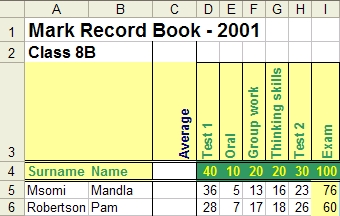
Consult the tip sheet
on Vertical
text if necessary.
Note that where text is
too long for a cell, Excel will display the full
text as long as there is nothing in the next door
cells.
Save the file as Record
Book
STEP 2
Add the names of 9 more
learners (up to row 15), and give them marks for
the various assessments (note that the maximum
for each assessment is in cells D4 to I4).. Save
the file.
STEP 3
Sort the names of the
class alphabetically according to the surname.
This tip may be useful:
- Sorting
data
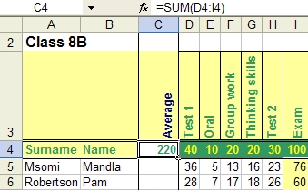
STEP 4
Enter a formula in C4
to calculate the total for all the assessments.
STEP 5
Select cells C5 and make
the number format Percentage with one decimal
place.
This tip sheet may help
you: Number
format
STEP 6
Insert this formula in
C5 to calculate a percentage for Mandla:
=SUM(D5:I5)/$C$4
What does this mean? We
are adding all the scores from D5 to I5, and then
dividing them by the total which is in C4. The
$ signs are added to make C4 an absolute
reference.
Note that the result is
automatically multiplied by 100 and the % sign
added because of what we did in step 5.
STEP 7
Autofill
this formula from cell C5 to cell C15.
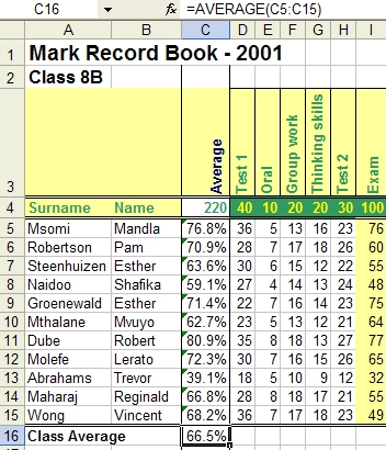
STEP 8
Use the AVERAGE function
to calculate an average percentage for the class
in cell C16.
STEP 9
- NEW USERS ARE NOT REQUIRED TO DO THIS STEP
The percentage we worked
out in C5 is OK, but it does not take any account
of WEIGHTING - ie how much different assessments
count. They are all just added together and converted
to a percentage.
We now need to make a
more sophisticated mark, one that is made up of
a term's work mark for tests (out of 25), and
continuous activities (out of 25).
Add the new column headings
as in J3 and J4, and then insert this formula
into J5: =(((D5+H5)/70)*25)+(SUM(E5:G5))/2
Autofill this formula
from J5 to J15.
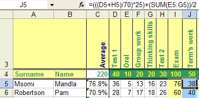
What does it mean? Let's
take it to pieces:
D5+H5
this adds the two test marks
((D5+H5)/70)*25 this
converts the test marks (out of 70 - so we divide
by 70) to a mark out of 25 (so we multiply by
25).
SUM(E5:G5) this adds
all the continuous marks
(SUM(E5:G5))/2 this
converts the continuous marks (out of 50) to a
mark out of 25.
=(((D5+H5)/70)*25)+(SUM(E5:G5))/2
this adds the two marks together to give a term
mark out of 50.
It looks complicated, but it isn't really. It
is just using the principles of BODMAS (see the
tip on simple formulae in the Formulas
tip sheet).
STEP 10
- NEW USERS ARE NOT REQUIRED TO DO THIS STEP
Let's take this one step
further. We now need to calculate a Term Mark
(the Exam added to the Term's Work Mark - to give
a mark out of 150), and then convert that to a
Percentage.
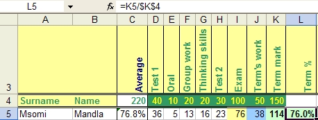
-
Add
the column headings as in K3 and K4, and L3.
-
In
K5, insert the following formula to add the
Exam mark with the Term's Work mark: =I5+J5.
-
Set
the number format of L5 to %.
-
In
L5, insert this formula: K5/$K$4 (why do we
have to make K4 absolute?)
-
Select
K5 and L5Autofill them both to K15 and L15.
Calculate
an average Term % in L16.
STEP 11
Copy the record book to another worksheet (not
a separate file) and enter the names and marks
of another class. To understand worksheets, refer
to the tip
sheet on worksheets.
STEP 12 - THIS IS AN ADVANCED STEP AND
IS FOR CONFIDENT SPREADSHEET USERS ONLY
If you would like to
get Excel to determine who has achieved competence
in this term, you can type the following formula
in M5 and autofill it to M15
=IF(L5>40%,"competent","working
towards competence")
-
IF
is a function that looks at a particular condition,
and then does one of two things depending
on whether the condition is met.
-
L5>40%
this is the condition - our "pass mark"
is 40% so we want the score in cell L5 to
be greater than 40%.
-
Note
the commas - they are very important!
-
"competent"
whatever comes after the first comma is the
result if the condition is met; because it
is a label (word) rather than a value (number)
it must be in quotes.
-
"working
towards competence" after the second
comma is the result if the condition is NOT
met.
The brackets are also very important!
STEP
13 (Optional)
If you have a very big
class, you might lose track of how many learners
you have. You can use the following functions
to count them:
=COUNTA(A5:A15)
this will count the number of entries in column
A. Note, we need to use COUNTA if we are counting
labels (words); COUNT only works with values (numbers).
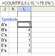
STEP 14 (Optional)
If you want to work out the symbol distribution
for your class, you can do the following:
-
In
J20 to J26 add the labels as shown
-
In
L20 type this formula: COUNTIF(L5:L15,">79.5%")
-
The
function COUNTIF will look at the range specified
(L5 to L15) and will check each cell in the
range against the criterion given after the
comma ">79.5%". Once again, the
brackets and comma are very important. The
quote marks "" are necessary because
we have specified more than just a number
on its own.
-
Can
you work out an appropriate formula to calculate
the number of B's etc? HINT: You can have
more than one COUNTIF in a formula.
Completion
of this activity
Save the record book.
Attach it to an e-mail to
your tutor (using the subject heading "Recordbook").
Use your
e-diary to make closing comments about
this activity. |