ICT and the Roles of the Educator - Optional Activity 5A: Activity 5: Spreadsheets for administrative purposes

Optional Activity 5A: An overview

This is an overview activity which aims to make you familiar with the key concepts of a spreadsheet. Before going further, you will need to open MS Excel* (Start-Programs-Microsoft Excel). You can use the buttons at the bottom of your screen (the task bar) to switch between Excel and these course notes in Internet Explorer (Alt+Tab also does this).

OVERVIEW

In this Overview activity, click on the blue headings of each new Concept, for an explanation of that Concept, before attempting the next step of the exercise provided for you in order to practise these basics.

CONCEPT 1: CELL

EXERCISE: STEP 1

In Excel, type the word Monday in cell A1. Note that "Monday" is now seen in the INPUT LINE also. The input line will always tell you what is in a cell. Also note that this cell A1 has a dark line around it. This indicates that the cell is selected.

CONCEPT 2: AUTOFILL

EXERCISE: STEP 2

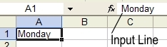
Drag with the autofill handle from cell A1 to cell G1. You should see this:

EXERCISE: STEP 3

Note that cell C1 does not show all of "Wednesday". This is because the column is too narrow. Click on C1, and look at the input line. Note that the full word is shown there. To fix the column width, take your mouse pointer to the line between the C and D column labels. It should look like this:

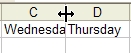Double-click, and Excel will make the column the right width for what is in it. This also works for Row Height.

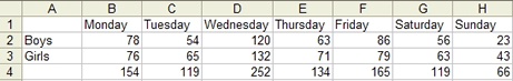
EXERCISE: STEP 4

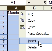
In this exercise we want to record the number of learners who visited a career exhibition during the week. We will need a separate row for boys and girls. But... we have not left space for this. So we have to insert a new row. Right-Click with you mouse pointer on the A column label. You should see this:

Click on insert to add a column to the left of the column which is selected.

Note, you can also use this right-click menu to Delete the selected column.

EXERCISE: STEP 5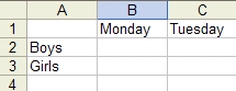

Column A should now be blank (if you correctly inserted a new column in Step 4). You can now type in "Boys" in A2 and "Girls" in A3.

EXERCISE: STEP 6

Now fill in the number of boys and girls who attended the exhibition each day.

HINT: try to train yourself to use the number keys on the right of your keyboard to enter numbers - it's much easier.

At this stage, note that there are two different kinds of information: words and numbers.

Excel call the words LABELS and the numbers VALUES.

CONCEPT 3: FORMULA

EXERCISE: STEP 7

Type the formula =B2+B3 in cell B4 and then push enter. You should see this when you click on B4:

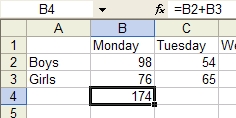Note: the result of the calculation, 174, is shown in cell B4, while the formula is shown in the input line.

This is a very important point: DO NOT type a calculated result (174 in this case) when you can use cell addresses in a formula to achieve a result. Why? Just say we discover that the number of boys on Monday was really 78. Change B2 to 78, and you will see B4 changes automatically. Magic!

EXERCISE: STEP 8

Here's another reason why you should type a formula instead of the actual number. We now want to get a total for each day. All you have to do is to use autofill to copy the formula from B4 to H4. More magic! This is what you should see:

Click on C4, D4 etc, and look at the input line for each. Note how Excel has incremented the cell addresses in each case to create a new, correct formula.

CONCEPT 4: RANGE

CONCEPT 5: FUNCTION

EXERCISE: STEP 9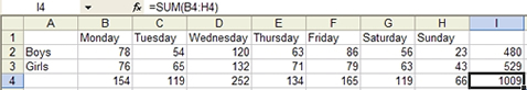

In cell I2, type this formula: =SUM(B2:H2) and then push enter. Autofill this formula to cells I3 and I4. You should see this:

Try changing any of the values, and you will see that all the formulae update automatically.

EXERCISE: STEP 10

We now want to do some calculations for the amount of money which the career exhibition has made. The entry fee was R3.50.

In cell A6, type the value 3.5 and push enter

With A6 selected, click this button (currency) on your tool bar

Note 1:
You may have to look for this button by clicking the very small triangle on the very right of the tool bar to see the hidden buttons. Once you have used it once, it will come onto the visible toolbar.

Note 2:
Iif your computer is set up with American settings, you will see a $ instead of the currency button.

You should see: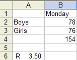

EXERCISE: STEP 11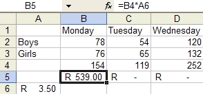

Now enter the formula =B4*A6 in cell B5 to work out the total amount of income on Monday.

Autofill the formula in B5 to I5. You should see this:

Why is Excel not able to work out the amounts for Tuesday, Wednesday etc? Have a look at the formulae which autofill created for you. What do you notice? To solve this problem, you need...

CONCEPT 6: ABSOLUTE REFERENCE - this is an advanced concept.

EXERCISE: STEP 12

This is an advanced concept. First-time users proceed to COMPLETION OF TASK

Type the formula =B4*$A$6 in cell B5 and then autofill. You should now see:

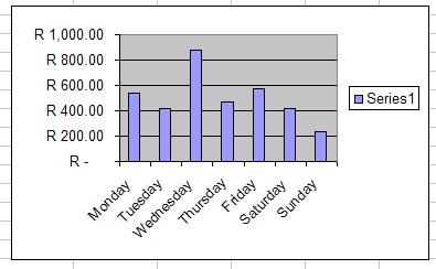
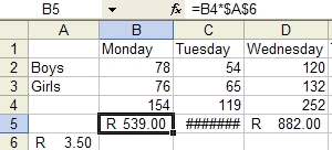If you get ####### in a cell, it means it is a value which is too long to display. You just need to adjust the column width (as in Step 3).

EXERCISE: STEP 13

This is an advanced concept.

The final step is to make a graph. When you make a graph, you must first select the values and labels you want to use in your graph. Drag (normal, not autofill) from B1 to H1 (Monday to Sunday), and then hold down the Ctrl key on the keyboard while dragging to select B5 to H5 (the total money for each day). (Using the control key allows you to select two areas not next to each other).

With the labels and values selected, you can click on the Chart Wizard button.

Just click the Finish button, and you should see: