Microsoft Excel 2007 - Pivot tables
How to create a Pivot Table
- Step 1: Create the Pivot Table
- Step 2: Select a first field to divide up your data
- Step 3: Select a second field to divide up your data further
- Step 4: Select a field to count
- Step 5: Working with a numeric field
- Step 6: Create a chart
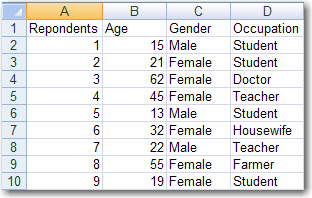
Enter data in columns with headings. There should be no blank rows or columns in between your data. Eg:
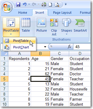
Step 1: Create the Pivot Table
Click on any cell which contains data.
Then, on the Insert tab, choose Pivot table from the Tables group.
A create pivot table popup will appear. The table/range is already filled because you clicked in a data cell before selecting pivot table. To change this click the red arrow and edit the data.
New Worksheet is automatically selected as the location to place the pivot table.
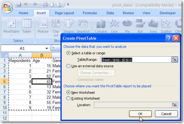
Click OK
Step 2: Select a first field to analyse your data
You should see a screen which looks like the following.
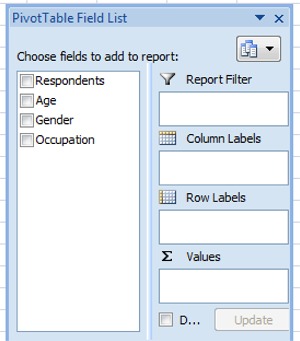
Note, Excel takes your column headings from your data and makes them into Fields. These are displayed in the Field List on the right hand side of the above image.
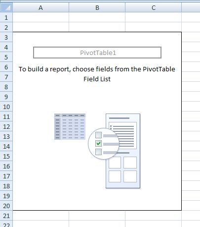
The above appears as a new sheet in your workbook. It is probably labelled Sheet 4 (or similar).
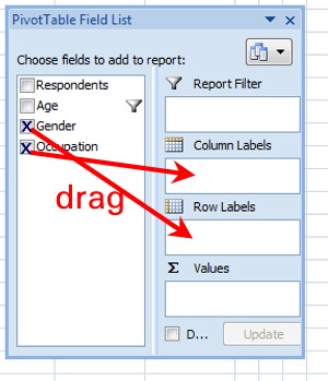
Choose a variable from the Field List (think about what data you want to see at a glance). For example if you wanted to count the number of male and female respondents, then you would want to select Gender.
Drag this variable into the Row labels area of the Field List.
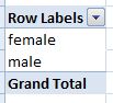
You should see something like this:
Step 3: Select a second field to divide up your data further
Choose one of the variables from the Field List that will help you further analyse the gender (e.g by occupation), and drag it to the Column Labels area of the Field List.
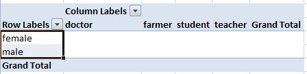
You should see something like this:
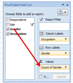
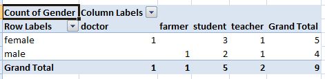
Step 4: Select a field to count
Drag the field that you wish to count (eg gender) to the Values area (marked with red arrow here):
You should see something like this:
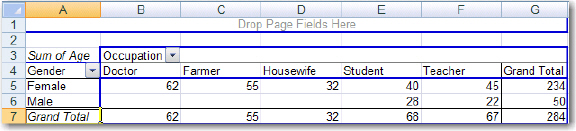
Step 5: Working with a numeric field
If you want to work with a numeric field (eg Age), you will need to:
Drag the "Count of..." button away
Drag the Numeric Field (eg Age) to this position
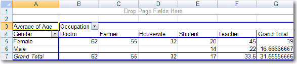
Right click the "Sum of..." button.
Select Summarize by, follow the arrow to the right and select Average
Click OK.
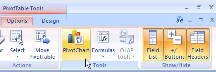
Step 6: Create a chart
Click on the Options tab and select Pivot Chart in the Tools group button to create a Graph
Click on the Chart Type button to select a different kind of graph
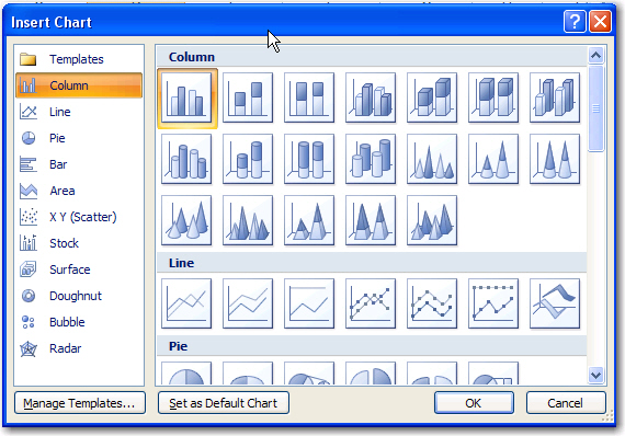
NOTE: You can choose different fields to graph by dragging a field away, and replacing it with another.
All Rights Reserved.