Graphics placed into Excel can use the Comments feature to label the picture or diagram.

First Set Margins

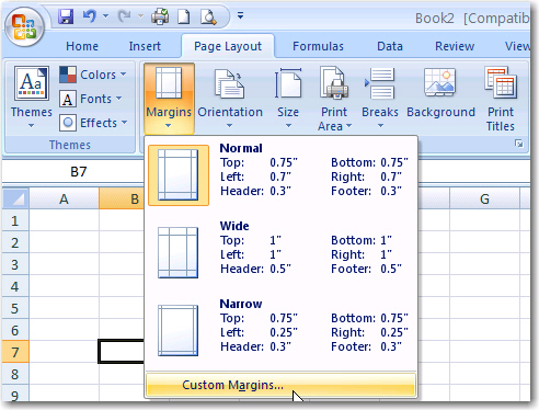
• On the Page Layout tab, select Margins from the Page Setup groups.
• Select custom margins
  
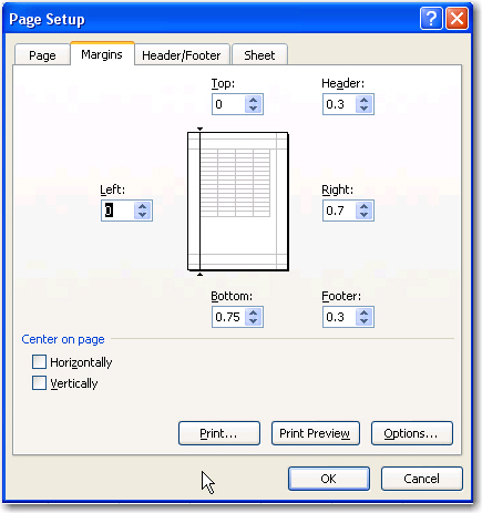
• Set the Top: to 0 and the Left: to 0.

Resize the Cells

The smaller the cells in the spreadsheet the more detailed the labeling can be.

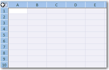
• Click in the area where the column and row headers meet. This will select the entire spreadsheet. (These are just example sizes, for more detailed maps, selecting smaller numbers is fine).
  

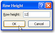
• From the Format menu, choose Row and then Height..

.

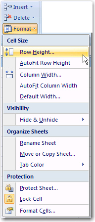
• Set the Row height: to 12 and click OK

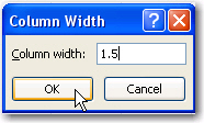
• From the Format menu, choose Column and then Width..

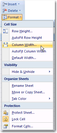
• Set the Column width: to 1.5 and click OK

• Click on any single cell to remove the highlighting

Put in the graphic

• On the Page layout tab, choose Background

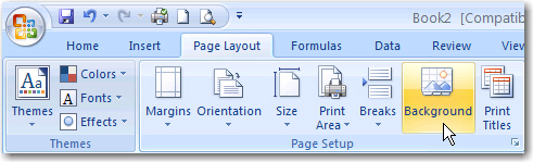
• In the dialog box, navigate to the desired graphic.
• Double click to select the graphic

Mask the Extra Images

• You will see that the background image is tiled. To eliminate this look:
• Highlight the first column you wish to hide by clicking the column heading. This will select the entire column (column T is highlighted in the example below)
• On the keyboard, hold down Ctrl and Shift, and press the right arrow key to select all columns to the right (of column T)

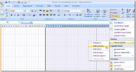
• From the Format drop down menu, choose Hide & Unhide and then Hide Columns. The extra columns will be hidden.
• Repeat the above process for hiding rows.
• Highlight the first row you wish to hide.
• Hold down Ctrl and Shift, and press the down arrow key.
• From the Format drop down menu, choose Hide & Unhide and then Hide Rows. The extra rows will be hidden.

Create the Comment Hot Spots/Insert Comments

• Click on one cell to highlight the spot on your picture where you want to put a hotspot/comment.
• From the Review tab, choose New Comment.
• Enter a comment that fits, or type a space to create a blank comment.
• Test your hotspot by moving the cursor slowly over the 'hot' spot in your picture. The comment should pop-up on the screen.

View All Comments

• To view all of the comments at the same time, from the Review tab, choose
  Show all Comments.
• To get rid of the all the comments, click Show all Comments again.

Edit the Comments

• In the Review tab, click in the comment box you want to edit.
• Select Edit comment, and then edit the text.

OR

• Move the mouse pointer over the cell were the comment to edit is located and right click the mouse button.
• From the pop-up menu, choose Edit Comment.
• Edit the text, and then click on any other cell to hide the comment again.

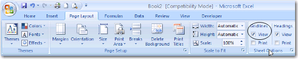
One Last Optional Item - Hide the Gridlines

• In the Page Layout tab, choose Gridlines from the Sheet Options group.
• The gridlines will disappear when you click the little white square(where you see the tick) to de-select the View gridlines.