Click here if you would like to open a starting spreadsheet to work through this example.  

1. Select all the cells to which you want to apply conditional formatting. Use Ctrl to select multiple columns of data.
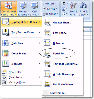
2. Click on Conditional Formatting in the Styles group
3. Click Highlight Cells Rules
4. Choose Equal To from the drop-down list

5.

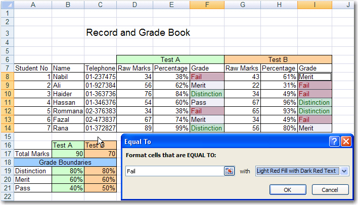
5. Click on the red arrow to select the data you want to shade. Then choose a colour pattern.

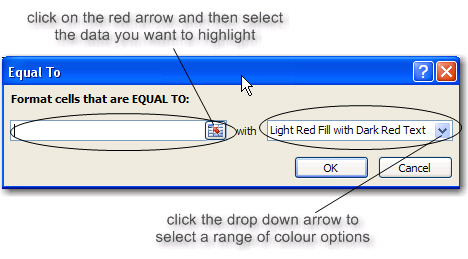
6. In this example, the selected data is "Distinction" and the colour pattern is "Green fill with Dark green text"

To set a second conditional format , repeat the above process.

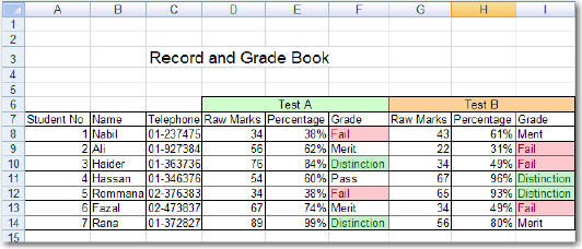
  Once you click OK, the worksheet should now appear as shown below.

TO EXPLORE
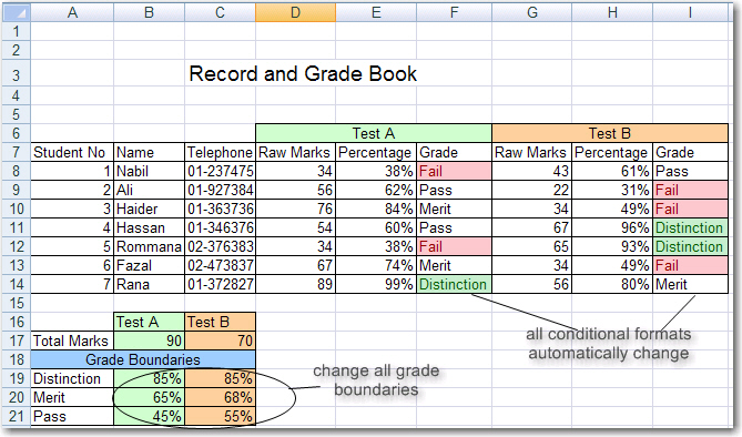
Explore the advantages of absolute referencing and setting up a separate section for grade boundaries. Let's say that you as a teacher decided to change the grades boundaries for both Test A and B. It's simple because all you have to do is change the values in the Grades boundaries section. All the rest is automatically generated. If you changed the Grade Boundaries as in the example below, all the cells which are dependent on these grade boundaries change automatically.

This demonstrates one of the main advantages of using a spreadsheet: they are DYNAMIC and FLEXIBILE